
Contents
- Executive Summary: The Climate Multiplier Thesis
- Modeling the Biomass Deficit in Oak Woodlands
- Vulnerabilities in Carbon Offset Calculations
- Resource Allocation: Powering the Data Engine
- Translating Data into Forest Management Policy
- Strategic Recommendations and Call to Action
Executive Summary: The Climate Multiplier Thesis
Sudden Oak Death is a climate crisis multiplier.
The disease kills tanoaks and coast live oaks that have accumulated carbon across decades. Once those trees decline, the woodland loses active sequestration capacity while dead biomass begins returning stored carbon to the atmosphere. The same event damages habitat, raises hazard-management costs, changes fuel structure, and weakens a living carbon reserve.
Regional conservation work initially centered on biodiversity loss. Rapid canopy collapse forced a broader accounting. Field observations showed that infected tanoaks can move from active carbon uptake to net carbon release within a few years of initial Phytophthora ramorum infection. Mature coast live oaks can also suffer structural failure within several years of bleeding canker development.
That timing matters. Climate plans often treat forests as durable assets over long crediting periods. Disease ecology works on a shorter clock.
Carbon Defense
Protecting mature, disease-resistant oaks preserves carbon already secured in wood. Replacing that stock through planting requires decades of successful growth.
Two conclusions follow. First, unchecked Sudden Oak Death mortality degrades the sequestration capacity of Pacific Coast woodlands. Second, carbon offset programs carry structural risk when their forecasts omit pathogen-driven biomass loss.
Woodland conservation therefore belongs inside climate planning, with management and prevention treated as carbon protection rather than a separate ecological concern.
Modeling the Biomass Deficit in Oak Woodlands
A useful carbon model starts with a physical question: how much living wood has disappeared from the canopy, and what happens to that material next?
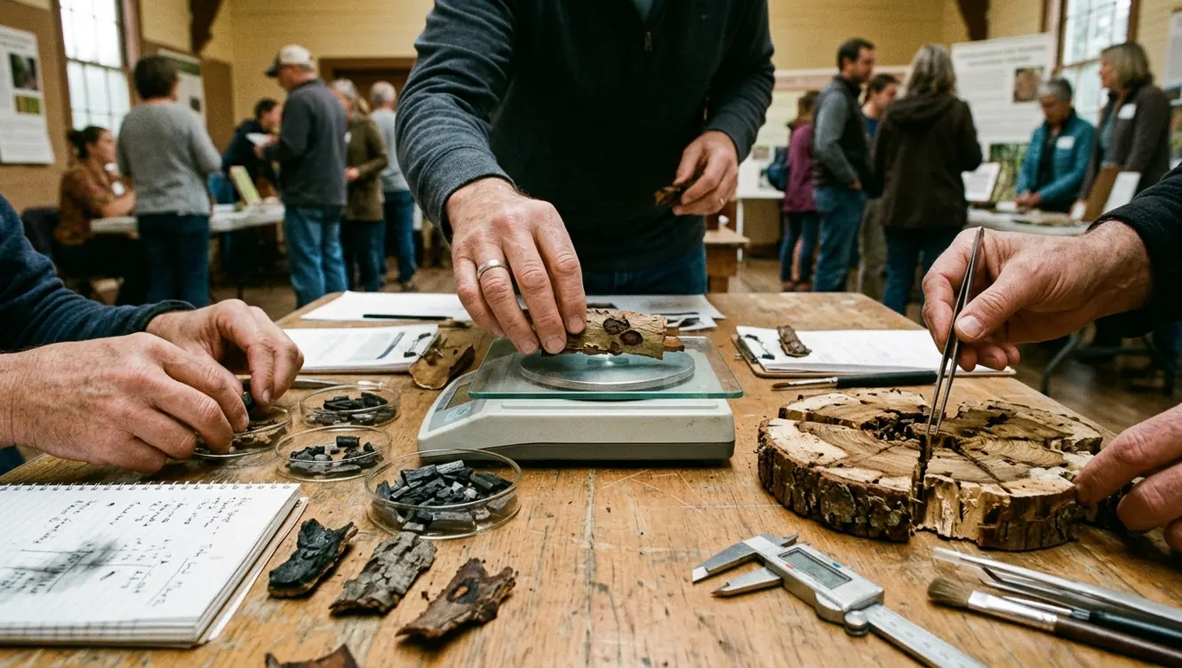
Regional forest inventories establish tree species, dimensions, density, and condition. Mortality observations then identify where tanoaks and coast live oaks have stopped adding biomass. Analysts can use established forest inventory data methodologies to structure those measurements, while localized SOD blitz surveys help reveal disease conditions that broad inventories may miss.
Reading Canopy Loss
Normalized Difference Vegetation Index imagery can flag a decline in canopy vigor across a large area. Its weakness is diagnostic precision: a satellite signal may register drought stress, fire damage, seasonal change, or pathogen-related decline in similar ways.
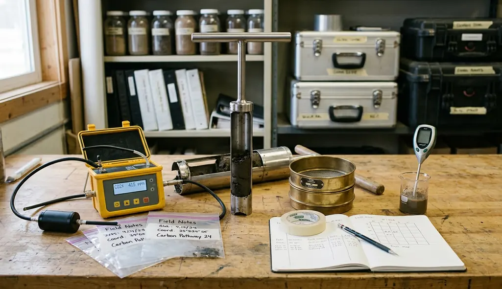
Low-altitude LiDAR offers a sharper view of canopy volume. Detailed scans over affected coastal watersheds can measure gaps, crown collapse, and changes in stand structure. Ground observations remain essential because a geometric canopy loss still needs a cause.
From Sink to Source
A living oak removes carbon dioxide from the atmosphere and stores part of that carbon in its trunk, branches, foliage, and roots. Infection interrupts new growth. Mortality ends active uptake. Decay then begins releasing the accumulated stock.
Standing dead tanoaks can lose structural integrity quickly, with much of their above-ground biomass decaying over roughly a decade. Microclimate changes the pace. Damp tanoak stands in the coastal fog belt generally decompose faster than coast live oaks on drier inland ridges.
Models should represent that sequence as a changing carbon balance rather than a single mortality event. A heavily affected stand may cross from sink to emitter when decomposition outpaces the growth of surviving trees and regeneration.
Academic Sources
Inventory protocols, species-specific biomass equations, mortality observations, and repeat canopy measurements should remain traceable in the model record. That audit trail lets land managers distinguish measured canopy loss from assumptions about future decay.
Vulnerabilities in Carbon Offset Calculations
Carbon offset projects establish a baseline for expected forest growth and expected loss. Credits depend on the difference between that baseline and the managed outcome. An underestimated disease threat distorts both sides of the calculation.
Historical fire-risk models can describe one major reversal pathway. They cannot represent localized Phytophthora ramorum spore pressure, host distribution, fog exposure, or the proximity of California bay laurel to valuable oaks. Projects that rely on fire history alone may consume their buffer pools prematurely when concentrated SOD mortality strikes a coastal parcel.
Why Static Baselines Break
A baseline often assumes that mortality will remain within a historical range. Pathogen outbreaks violate that assumption because transmission depends on current host conditions and local weather. Two neighboring parcels may face very different exposure when one contains abundant foliar hosts near mature oaks.
Offset registries commonly reserve a share of credits against unintentional reversals. Severe localized mortality can exceed that protection. The accounting problem appears before every dead tree decomposes: projected sequestration disappears immediately, while stored carbon enters a longer release pathway.
Root Carbon Gap
Current sequestration models primarily track above-ground biomass. Root-system decay remains under longitudinal observation and may change long-term projections.
This uncertainty should shape model boundaries. It does not justify omitting known canopy mortality. Above-ground measurements can support present decisions as long as the model identifies which pools it measures and which remain under study.
Future valuations need dynamic disease-risk variables. Useful inputs include confirmed infections, susceptible host density, nearby bay laurel, local moisture patterns, and repeat observations of canopy condition. Updating those variables turns disease risk into a monitored condition instead of a fixed assumption.
Resource Allocation: Powering the Data Engine
High-resolution disease mapping depends on many small observations collected at the right time. Citizen science supplies that reach.
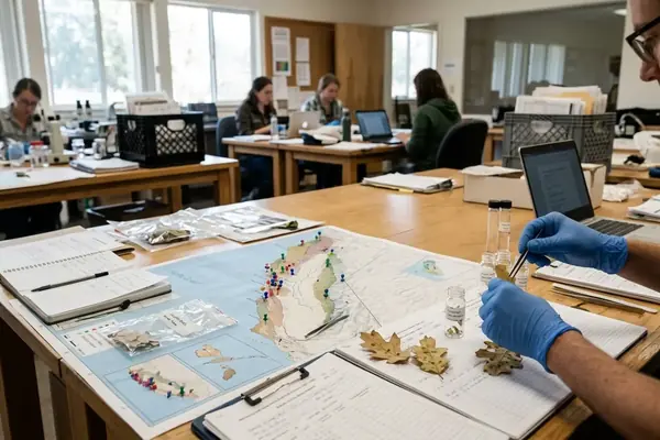
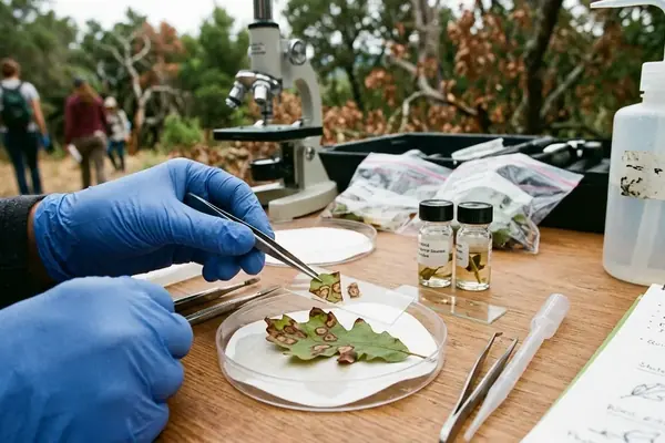
During sod blitz surveys, volunteers examine local trees, record field context, and collect symptomatic leaf tissue during the spring sporulation window. Samples must enter a cold chain immediately and reach pathology processing quickly. Delayed or poorly handled tissue can degrade before testing, weakening the map built from it.
What Funding Must Cover
A transparent impact report should connect community funding and conservation grants to four operational functions:
- Seasonal field coordination: selecting survey locations, preparing collection materials, and training volunteers in consistent sampling.
- Sample integrity: chilling, transport, intake, and timely pathology processing.
- Spatial analysis: linking confirmed results with host distribution, canopy condition, and localized disease risk.
- Public reporting: returning usable maps and management guidance to land trusts, homeowners, and conservation authorities.
This breakdown keeps the financial story tied to evidence production. A collection kit has limited value without correct timing. A test result has limited reach without location data. A risk map has limited conservation value unless land managers can act on it.
Hours Become Evidence
Volunteer effort translates into mapped observations through a strict chain: locate symptoms, collect suitable tissue, document the site, preserve the sample, process it, and return the result to the spatial record.
Sampling Clock
Concentrate volunteer deployment in the peak spring window. Seasonal focus protects sample quality and directs limited coordination time toward periods when viable cultures are most likely.
The measured impact is finer local coverage than a small professional field team could gather alone. That coverage helps carbon models identify where mortality risk clusters around mature stands. It also gives regional climate policy a clearer view of where stored forest carbon faces immediate biological pressure.
Translating Data into Forest Management Policy
Policy should protect living carbon before agencies spend scarce conservation funds on widespread hazard removal.
Large-scale removal can reduce immediate safety concerns around roads, structures, and trails, yet it does little to slow transmission when infectious foliar hosts remain in place. Proactive management focuses on high-value oak stands, nearby disease reservoirs, and the conditions that support spread.
Choose Stands by Carbon Value
Land managers should begin with mature tanoaks and coast live oaks that retain healthy crowns, occupy important woodland corridors, and represent substantial standing biomass. Large mature oaks deserve priority because their accumulated carbon cannot be replaced by saplings within a normal planning cycle.
Resistance mapping adds another filter. A mature oak that remains healthy within an exposed watershed may offer both current carbon value and useful evidence of natural resistance. Protecting clusters of such trees strengthens woodland conservation while improving the next round of disease modeling.
Containment at Stand Scale
Localized sanitation targets California bay laurel, the primary foliar host, close to high-value coast live oaks. Removing bay laurel within a tightly defined area can reduce nearby inoculum pressure while avoiding indiscriminate clearing across the woodland.
Dry-season phosphonate treatment provides another targeted option for selected trees because bark conditions favor absorption during that period. Treatment records should include tree condition, timing, location, and follow-up observations so managers can judge whether the intervention preserved canopy function.
Protect First
Rank stands by mature biomass, exposure, and evidence of resistance. Direct sanitation and treatment toward the places where carbon loss would be hardest to replace.
Localized quarantine practices also matter. Soil, leaves, and plant material can move the pathogen beyond an affected site. Clear handling rules for crews, volunteers, and property owners connect field containment with the larger carbon objective.
Strategic Recommendations and Call to Action
Regional climate action plans should name forest pathogens as a direct threat to carbon permanence. That change would place SOD monitoring beside fire, drought, and land conversion in forest-risk budgets.
The immediate funding priority is localized resistance mapping in coastal watersheds where mature oaks remain healthy under disease pressure. Over the next several planning cycles, authorities can pair that mapping with targeted sanitation, seasonal treatment, repeat canopy measurements, and community sampling.
A Shared Monitoring Network
Land trusts can identify high-biomass stands and provide repeat access. Homeowners can watch susceptible trees, join seasonal sod blitz surveys, and report symptoms early. Field coordinators can maintain sampling protocols and connect confirmed results to management maps.
Each participant fills a different gap. Together, they create the local evidence needed to protect mature trees before canopy collapse appears in regional imagery.
Conservation authorities should fund localized SOD resistance mapping ahead of generic reforestation and use those maps to defend mature oaks already holding decades of carbon.



Your Thoughts
No comments.
Leave a Comment